From Smooth to Jagged

From Smooth to Jagged How Mathematics Learned to Map Reality

"As far as the laws of mathematics refer to reality, they are not certain; and as far as they are certain, they do not refer to reality." - Albert Einstein, Geometry and Experience

"Clouds are not spheres, mountains are not cones, coastlines are not circles." - Benoit Mandelbrot, The Fractal Geometry of Nature

July 2026 Nick Alonso

I. Introduction: The Equations Reality Writes

Mathematics did not grow by accident. Nearly every major tool in the analyst's kit was invented because reality posed an equation of change, a differential equation, that the existing mathematics could not solve. Heat flowing through a cannon barrel, a comet swinging past Jupiter, pollen jittering in water, static crackling on a telephone line: each one forced mathematics to grow a new limb. This paper follows four of those limbs in the order reality demanded them, from the perfectly smooth world of Taylor series to the jagged, fractional world of fractals.

It ends with a personal story. Years ago I wrote a letter to a mathematician listed on the Yale faculty. His reply changed how I read equity markets, but that story comes at the end, where it belongs.

II. The Taylor Series: Predicting the Curve

Classical calculus assumes a smooth world, and in a smooth world the Taylor series is the ultimate predictive engine. Its claim is bold: if you know everything about a single point on a well-behaved curve, every derivative, layer by layer, you can reconstruct the entire curve from that one point.

The layers of change. In physics the derivatives form a kinematic sequence, each one a deeper layer of how motion changes. Position tells you where the object is; velocity, how position changes. Acceleration is the change in velocity, and the third derivative, jerk, is the change in acceleration. Jerk is the one you feel as the sudden snap of your neck when a driver stomps the brakes. Engineers even name the fourth derivative (snap) and design around it: elevator and roller coaster designers explicitly limit jerk and snap because the human inner ear feels those layers, not speed itself. A well-tuned elevator is a Taylor series you can ride.

The equation. The series takes the local information at a point a and projects it outward to predict the value at x:

f(x) = Σ [ f⁽ⁿ⁾(a) / n! ] (x − a)ⁿ, summed from n = 0 to ∞

Why symmetry does the heavy lifting. The quiet magic of Taylor expansions is how often the terms cancel. At any stable equilibrium, the bottom of any valley, the first derivative is zero by definition. The first surviving term is the quadratic one, which is why a pendulum at rest, a spring, a chemical bond, and a suspension bridge all obey the same mathematics near equilibrium. Nature looks like a parabola at the bottom of every valley, not by coincidence but by symmetry. The same trick appears with even and odd functions: the symmetry of cosine kills every odd-powered term before you lift a pencil. Once you see these cancellations, whole fields of physics stop looking like separate subjects and start looking like one expansion with different constants.

A caution for the fine print: the full reconstruct-everything claim holds only for analytic functions. The classic counterexample is e^(−1/x²), a function perfectly smooth at zero whose Taylor series there predicts nothing at all. Even the smooth world keeps some secrets.

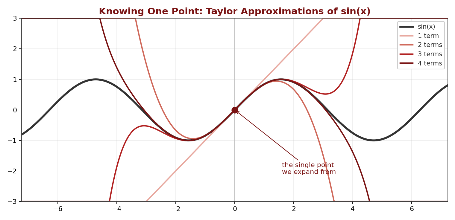
Figure 1. Knowing one point. Each added term of the Taylor series hugs sin(x) farther from the expansion point, and every approximation eventually peels away. Prediction radiates outward from local knowledge, with a finite reach.

The comet that made it famous. In 1758, Alexis Clairaut and two collaborators spent months grinding through perturbation series to predict when Halley's comet, tugged off schedule by Jupiter and Saturn, would round the Sun. Clairaut announced a date; the comet arrived within roughly a month of it, the first great public demonstration that knowing the derivatives means knowing the future [2]. It remains the founding legend of predictive modeling.

The differential equation underneath. Why did the series exist at all? Because most differential equations have no clean closed-form solution. The Taylor series is how you solve an equation of motion locally, one derivative at a time, when no formula exists. It was the first limb mathematics grew to reach reality, and it works beautifully as long as reality stays smooth.

III. The Fourier Transform: Un-blending Chaos

Where calculus studies smooth curves, Fourier analysis attacks messy aggregates and un-blends them. Its claim: essentially any physically realistic signal, however chaotic it looks, can be rebuilt by adding together simple, endlessly repeating sine and cosine waves.

Two ways of seeing. The time domain is the chronological shape of a signal, the physical wiggle of a guitar string over one second. The frequency domain is the ingredients list: it ignores when things happened and reveals which pure notes exist inside the noise, and how loudly. Same information, two languages.

The equation. The transform acts as a resonance probe, sweeping across all time and multiplying the messy signal by perfect waves to see what matches:

X(f) = ∫ x(t) e^(−i2πft) dt, integrated over all t

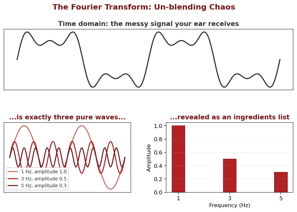
Figure 2. Un-blending. The messy signal on top is exactly the three pure waves below it, and the frequency domain reads off the recipe: which notes, at what strength. Your cochlea performs this decomposition mechanically, before your brain gets involved.

You are running one right now. The best example is not in a lab. The cochlea in your inner ear is a physical Fourier transform: a coiled strip in which each position resonates with one frequency. When a chord reaches your ear as a single mangled pressure wave, the cochlea splits it back into notes before your brain ever gets involved. That is why you can pick a single voice out of a crowded room, and it is the same decomposition running inside noise-canceling headphones and song-recognition apps.

The man nobody believed. Joseph Fourier went to Egypt with Napoleon, came home obsessed with heat, and in 1807 presented a memoir claiming any temperature profile could be built from waves. Lagrange and Laplace, the two most powerful mathematicians alive, found the claim absurd, and publication was effectively held up for years. Fourier kept going, publishing his full theory in 1822 [3]. He was right, and it took the field decades of work, including the discovery of strange wrinkles like the Gibbs phenomenon at sharp edges, to establish just how right.

The differential equation underneath. Fourier did not invent his series as abstract mathematics. He built them for one purpose: to solve the heat equation, the partial differential equation governing how temperature spreads through a solid. The waves were the only shapes the equation treated simply, so he expressed everything else in terms of them. Reality posed the equation; the transform was the limb that reached it.

A bridge to another paper in this library: Shor's algorithm, the quantum method for breaking RSA encryption, is at its heart a Quantum Fourier Transform hunting for the period of a function. The same idea, un-blend the chaos and read off the frequency, does the work in both worlds.

IV. Stochastic Calculus: Modeling the Jagged Edge

Everything so far assumes the curve is smooth enough to differentiate. In 1827 the botanist Robert Brown looked through his microscope at pollen grains suspended in water and watched them jitter, endlessly and without cause [4]. No one could explain it for nearly eighty years, until Einstein showed in 1905 that the jitter was the statistical signature of invisible molecules colliding with the grains, an argument so quantitative it effectively settled the existence of atoms [5].

The path that broke calculus. A Brownian path is continuous but so jagged that it has no derivative anywhere. Zoom in and it never smooths out; there is no velocity to speak of. Ordinary differential equations simply break on such paths. Standard calculus builds on dx and dt, infinitesimal steps in space and time. Stochastic calculus adds a third object, dW, the increment of a Wiener process, which is a formalized random shock. Kiyosi Itô worked out the rules for this new object in the 1940s [7], and his lemma, the stochastic chain rule, is the bridge that lets calculus survive contact with randomness:

df = ( ∂f/∂t + μ ∂f/∂x + ½σ² ∂²f/∂x² ) dt + σ (∂f/∂x) dW

The dt term is the deterministic drift, the direction the system is trying to go. The dW term is the volatility, the jagged noise throwing it off course. The strange extra piece, the half-sigma-squared term, exists only because randomness accumulates differently than smooth change. Volatility is not a flaw bolted onto the model; it is written into the calculus itself, the price of admission for modeling anything real.

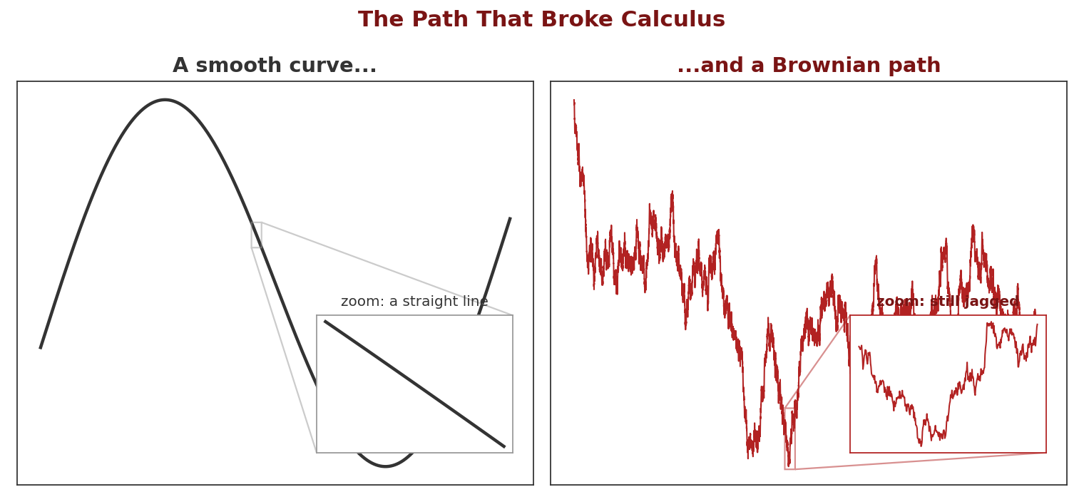
Figure 3. Why a new calculus. Magnify a smooth curve and it flattens into a straight line, which is what a derivative is. Magnify a Brownian path and it stays exactly as jagged, at every scale, forever. There is no line to find, so ordinary calculus has nothing to grip.

The graduate student who was too early. Here is the part your finance colleagues rarely hear. In 1900, five years before Einstein's paper, a doctoral student in Paris named Louis Bachelier wrote down the random walk model, not for pollen but for prices on the Paris Bourse [6]. His thesis, Théorie de la Spéculation, contained the mathematics of Brownian motion before physics had it. It was politely graded and thoroughly ignored for half a century, until the statistician Jimmie Savage mailed postcards to a list of economists asking whether anyone had heard of this Bachelier. Paul Samuelson found the thesis in the MIT library, and modern quantitative finance fell out of it: Itô's calculus applied to Bachelier's idea yields the Black-Scholes equation that prices options today [8].

The differential equation underneath. Black-Scholes is itself a differential equation, but of the new kind: a stochastic one, an SDE rather than an ODE. Reality's jaggedness did not just resist the old equations; it forced an entirely new species of them into existence. That is the pattern of this paper repeating: the tool is born the moment the old mathematics fails.

V. Fractals: The Geometry of the Infinite

The final limb abandons Euclid entirely. Circles, squares, and smooth lines describe almost nothing in nature; coastlines, blood vessels, lightning, and tree branches are rough at every scale. Fractal geometry is the mathematics of that roughness, and its founding insight is that staggering complexity can be generated by absurdly simple rules, repeated.

Noise on the line. Benoit Mandelbrot did his defining work not at a university but at IBM, studying bursts of random errors on telephone lines used for data. He noticed the errors had the same clustered structure at every timescale: hours looked like days, seconds looked like hours [10]. The pattern was self-similar, and once he had the eye for it, he saw the same signature everywhere, including in a hundred years of cotton prices.

The equation. His most famous object comes from iterating one line of algebra on the complex plane, feeding each output back in as the next input:

zₙ₊₁ = zₙ² + c

For each starting point c, one of two fates unfolds: the sequence stays bounded forever, sometimes settling to a point, sometimes cycling, sometimes wandering without escape, or it flies off to infinity. The Mandelbrot set is the collection of points that stay home. Its boundary, the infinitely intricate filigree between staying and escaping, is where the fractal lives: an edge so sensitive that two starting points closer than any measurement can distinguish end up with opposite destinies.

Between dimensions. The idea I find most fascinating is that fractals occupy fractional dimensions, and this is measurable, not metaphorical. Halve your ruler and the measured length of a smooth line grows by a factor of 2; a filled area grows by 4. Measure the coast of Britain with an ever-shorter ruler and it grows by roughly a factor of 2 raised to the power 1.25 [9]. The coastline is genuinely a 1.25-dimensional object, too wrinkled to be a line, too empty to fill a plane. Your lungs run the same trick from the other side, folding roughly a tennis court of gas-exchange surface into your chest, a surface so crumpled its dimension approaches 3. Fractional dimension is how nature fits infinity into finite space.

The differential equation underneath. An iterated map like z² + c is the discrete cousin of a differential equation: a dynamical system stepped forward in time. The fractal boundary is the map of where that system's behavior becomes infinitely sensitive to its starting point, which is to say, it is a picture of exactly where prediction fails. The first limb in this paper promised that knowing a point means knowing the future. The last limb draws, in infinite detail, the boundary of where that promise breaks.

VI. The Last Limb: Markets and a Letter

Now the story from the introduction. Years ago, after moving to Boston, I looked up Benoit Mandelbrot and found him listed on the Yale faculty. I was headed to New Haven and wrote to ask whether I could meet him. His reply surprised me twice: he was not in New Haven at all, he lived in Cambridge, and when I returned we could meet for coffee. I have long since lost the correspondence, but I remember its substance clearly. He was in the last stretch of his life, and he passed away soon after. The coffee never happened.

The reading I did to prepare for a meeting that never came did the work instead. His book on markets, and Fractals and Scaling in Finance [11][12], materially changed how I look at equity markets. Markets have never seemed random to me, exactly, but they have never seemed measurable by our standard tools either. Mandelbrot gave that intuition a precise form. A pure random walk, the assumption buried inside Bachelier, Black-Scholes, and most of the modern toolkit, traces a path with fractal dimension of exactly 1.5 and politely thin tails. Mandelbrot's claim was that real price series live at some other roughness. Volatility clusters, calm begets calm, wildness begets wildness, and the pattern looks the same on a one-minute chart as on a decade chart, a structure he measured with what is now called the Hurst exponent [13]. When markets produce moves the standard models call impossible, it is not because reality misbehaved. It is because we measured a fractional object with integer tools.

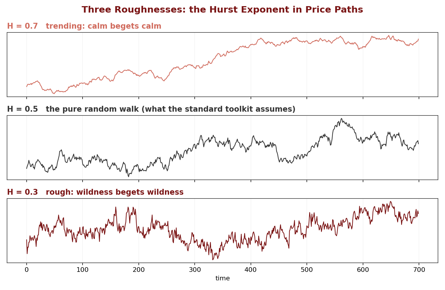
Figure 5. Three roughnesses. Simulated price paths at three Hurst exponents. The middle panel is the pure random walk assumed by the standard toolkit, with fractal dimension exactly 1.5. Real markets live at some other roughness, and the difference is measurable.

That is the thesis of this whole paper, arriving in person. Reality posed equations; mathematics grew limbs to reach them, from smooth Taylor expansions to the heat equation's waves, to a calculus for jagged paths, to a geometry for objects between dimensions. The last limb is the one I now use every working day. I never got the coffee, but I got the lens.

References

• [1] Taylor, B. (1715). Methodus Incrementorum Directa et Inversa. London.
• [2] Clairaut, A.-C. (1759). "Mémoire sur la comète de 1682." Journal des Sçavans, Paris.
• [3] Fourier, J. (1822). Théorie analytique de la chaleur. Firmin Didot, Paris.
• [4] Brown, R. (1828). "A brief account of microscopical observations on the particles contained in the pollen of plants." Philosophical Magazine, 4, 161-173.
• [5] Einstein, A. (1905). "Über die von der molekularkinetischen Theorie der Wärme geforderte Bewegung von in ruhenden Flüssigkeiten suspendierten Teilchen." Annalen der Physik, 17, 549-560.
• [6] Bachelier, L. (1900). "Théorie de la spéculation." Annales scientifiques de l'École Normale Supérieure, 17, 21-86.
• [7] Itô, K. (1944). "Stochastic Integral." Proceedings of the Imperial Academy, Tokyo, 20, 519-524.
• [8] Black, F., & Scholes, M. (1973). "The Pricing of Options and Corporate Liabilities." Journal of Political Economy, 81(3), 637-654.
• [9] Mandelbrot, B. (1967). "How Long Is the Coast of Britain? Statistical Self-Similarity and Fractional Dimension." Science, 156(3775), 636-638.
• [10] Mandelbrot, B. (1982). The Fractal Geometry of Nature. W. H. Freeman, New York.
• [11] Mandelbrot, B., & Hudson, R. L. (2004). The (Mis)Behavior of Markets: A Fractal View of Risk, Ruin, and Reward. Basic Books, New York.
• [12] Mandelbrot, B. (1997). Fractals and Scaling in Finance: Discontinuity, Concentration, Risk. Springer, New York.
• [13] Hurst, H. E. (1951). "Long-Term Storage Capacity of Reservoirs." Transactions of the American Society of Civil Engineers, 116, 770-799.