Portfolio Manager & Global Strategist

The Resolution of Reality A Primer on Quantum Computing "There is no need to build a labyrinth when the entire universe is one." - Jorge Luis Borges, from The Aleph July 6th, 2026 (revised September 2026) Nick Alonso

I. The Problem of Scale: The Lock on the World

Every time you send a credit card number or a private message across the internet, you are relying on a mathematical lock known as RSA Encryption Appendix A: The Mathematics of RSA. [1] The security of this lock rests on a single, widely believed assumption: that factoring large integers is computationally infeasible for classical computers. To create a lock, a computer takes two huge prime numbers and multiplies them together to create a massive "Public Key." To break the code, a hacker must work backward, taking that massive number and splitting it back into its two original factors. Without knowing the prime numbers, the hacker is working blind. There is no efficient mathematical map to guide them toward the answer; even the most advanced classical methods amount to a search far too long to ever finish. While the solution is simple, the difficulty lies in the scale. Modern RSA keys are typically 2048 bits long. Written out, this is a number roughly 617 digits long. The number of atoms in the observable universe is roughly 10^80. The total pool of numbers to check for a 2048-bit key is roughly 10^617. This represents a hard physical limit on computation. As the classic analogy goes: even if you turned every atom in the observable universe into a supercomputer and let them run for the entire age of the cosmos, they would still fail to make a dent in the problem. [Note: Strictly speaking, a hacker only needs to search up to the square root of the number. However, even with that reduction, the search space remains exponentially larger than the physical resources of the universe.]

Figure 1. The scale of the problem.

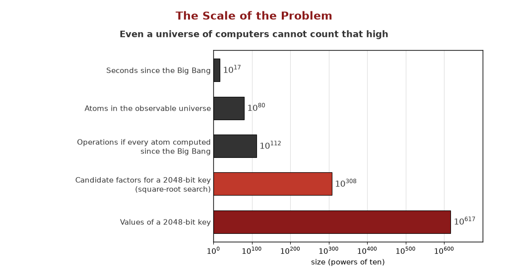
Figure 1. The scale of the problem. Plotted by exponent, the physical resources of the universe (dark) do not come close to the number of candidates a 2048-bit key hides (red), even after the square-root shortcut.

That scale sets up the argument of this primer. A quantum computer does not escape the limit by counting faster. It escapes it, when it can, by exploiting structure the problem already has. Where that structure is the physics of the problem itself, the advantage is largest. Where there is no structure to exploit, the advantage mostly disappears. The sections that follow build the physical picture; Section VIII returns to this gradient.

II. The Classical Reality: The Physical Cost

Why is this problem so hard for a classical computer? Because each classical bit holds one definite value at a time, a classical machine can evaluate only one candidate factor per operation. It can do this extremely fast, but the count of candidates (10^308 even after the square-root shortcut) is what defeats it, not the speed of any single check. Information is physical. A number is stored in bits, a bit is implemented in a transistor, and each candidate must be written into those transistors, tested, and cleared before the next one can be loaded. That physical cost is real, but it is not the bottleneck. The bottleneck is sequence. Every guess is a separate event, and there are more guesses than there are events available in the universe. Note: Bitcoin mining (Proof of Work) is the same guess-and-check procedure applied to a hash function. Miners load candidate numbers one at a time until one produces a hash below a target, and the network is secured by the cost of that search. The difference from factoring matters for what follows: a hash has no hidden structure to exploit, while modular exponentiation does. That difference is exactly what separates the problems a quantum computer can accelerate from the ones it cannot (Section VIII).

III. The Quantum Shift: Physics Solving Physics

Quantum computing approaches this problem in a fundamentally different way: it uses the laws of physics to solve the problems of physics. If the classical approach is like looking for a specific grain of sand by checking each one, the quantum approach is like placing that sand on a metal plate (Chladni plate) and vibrating it. You don't need to touch the sand. Through the application of specific frequencies, you can get the sand to naturally move away from the "wrong" spots, revealing the "right" spots where the answer lies. A quantum computer does not examine solutions individually. Instead, it represents many possibilities at once and manipulates them as a single physical system to reveal the right answer. The Qubit: The quantum equivalent to the classical bit is called a qubit. Like a classical bit, the qubit is a physical object and ultimately produces a 0 or a 1 when finally measured. However, before measurement, the qubit's physical state exists in a combination of possibilities between 0 and 1. In simple terms, the qubit is not committed to being a 0 or a 1 yet; both outcomes remain physically possible until the act of measurement forces a choice. Because each qubit is suspended in this state of possibility, we can manipulate them using physical laws. By applying specific forces (the algorithm), we coerce the system to resolve into the exact sequence of 0s and 1s that represents the correct answer. To understand how this works in more detail, we need to look more closely at the physics involved. In the next sections, we will introduce three key concepts that form the foundation of quantum computing: superposition, entanglement, and coherence.

IV. Superposition: Reality, Not Theory

The idea that a qubit can exist in a "combination of possibilities" has a name: superposition. Superposition sounds abstract, but it describes a real physical behavior. Before a quantum system is measured, it does not need to commit to a single outcome. Multiple outcomes remain physically possible at the same time. This behavior has been observed and tested repeatedly in experiments, the most famous of which is the Double-Slit Experiment. [2] Young's Double Slit Experiment: Imagine you are firing individual particles (like electrons) at a barrier with two narrow slits. Behind the barrier is a detector wall that records where each particle lands. The Classical Expectation: If particles acted like tiny bullets, they would pass through either the left slit or the right slit. You would expect to see two simple piles of hits on the back wall, directly behind the openings. The Quantum Reality: That is not what happens. Instead of two piles, the particles land all over the back wall in a series of alternating bright and dark stripes known as an interference pattern. This pattern is identical to what happens when water waves pass through two openings. The waves ripple out, overlap, and interfere with each other, sometimes combining to make a bigger wave (bright stripe), sometimes canceling out (dark stripe).

Figure 2. The double slit.

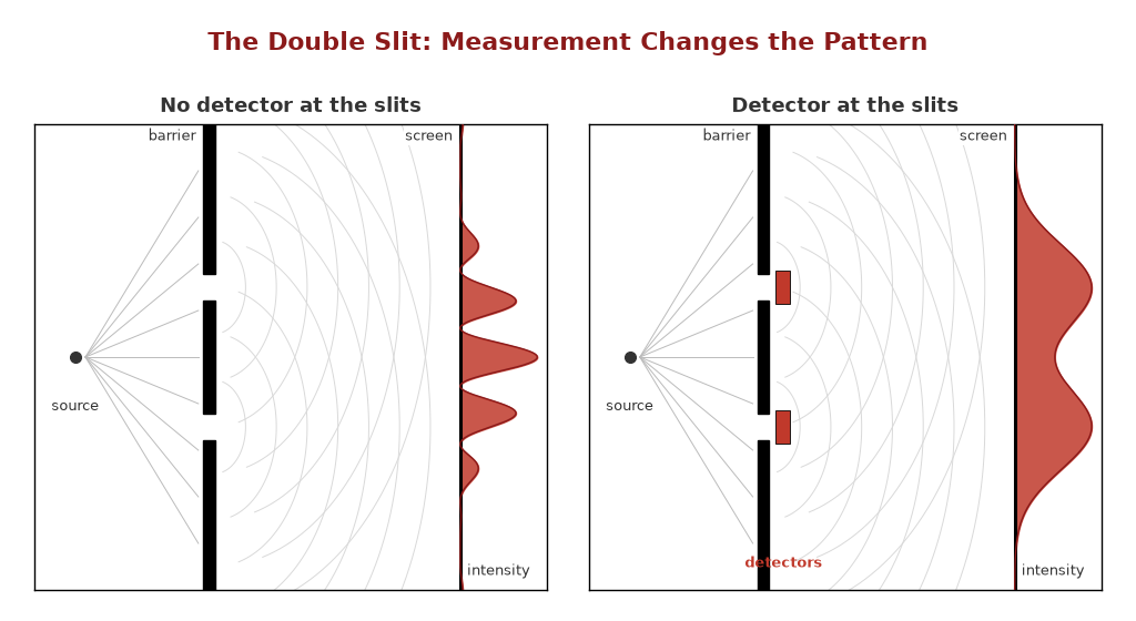
Figure 2. The double slit. Left: with no detector at the slits, the wall records an interference pattern. Right: a detector that records which slit each particle used destroys the pattern and leaves two piles. The act of measurement changes the result.

The Role of Measurement: However, this wave-like behavior is fragile. The key lesson from the experiment is that measurement, or interaction, changes the result. If you place a sensor at the slits to see which path the particle actually took, the wave collapses. The interference pattern disappears, and you are left with two simple piles of particles. In this sense, the detector forces the quantum particle, which was in a superposition of "left" and "right", to strictly become one or the other.

Connection to Computing: A classical bit must choose one path. But a qubit in superposition is the wave passing through both. It explores the pathway of 0 and the pathway of 1 at the same time. We can think of the back wall as the landscape of all possible answers. The slits represent the qubits. The interference pattern on the wall represents the probability of finding the answer in a specific spot. The more qubits we have, the more 'slits' we open, and the more of the wall gets exposed. As long as we have enough slits (qubits), we can see the entire 'wall' of possible answers. In our RSA encryption example, the slits represent the qubits that will eventually reveal the 0s and 1s of the correct encryption key. The next step is to make sure that all of these qubits are aware of each other, so that they can work together to represent the complex pattern of the solution as a single, unified system that encompasses all possible answers. This is called entanglement.

V. Entanglement: When Systems Stop Being Separate

Superposition allows a single qubit to explore two possibilities at once. But meaningful problems require checking trillions of possibilities. To do this, we need multiple qubits working together as a single team. This linking is called entanglement. Appendix B: Entanglement and Breaking the Logic Barrier The "Single Entity": When qubits are entangled, they stop acting as independent objects and behave as a single physical system. This is much more than a simple physical connection. Entanglement is measured by correlations, and in quantum mechanics, the correlation among entangled objects is significantly stronger than any classical interpretation would allow. In fact, these correlations are so strong that, assuming the objects stay in superposition, they will continue to influence each other regardless of the distance between them, even if separated by the physical expanse of the universe. (Importantly, this link cannot be used to send messages faster than light; it reveals itself only in the correlations between measurements.) This is where Einstein's famous objection about "spooky action at a distance" came from. Returning to the Double Slit: How does this help us solve the encryption problem? We can visualize the power of entanglement by returning to our Double Slit Experiment. 1 Qubit = 2 Slits: A single qubit in superposition is like a barrier with two slits. The wave passes through both (representing 0 and 1) simultaneously. Entanglement = Adding Slits: When we entangle qubits, we are mathematically adding more "slits" to the barrier. Two entangled qubits create 4 possible paths (00, 01, 10, 11). Three entangled qubits create 8 paths. With roughly 2,000 entangled qubits, we create a barrier with 10^617 slits. (In practice, Shor's algorithm uses roughly double that, about 4,000 logical qubits, to read the pattern reliably Appendix D.)

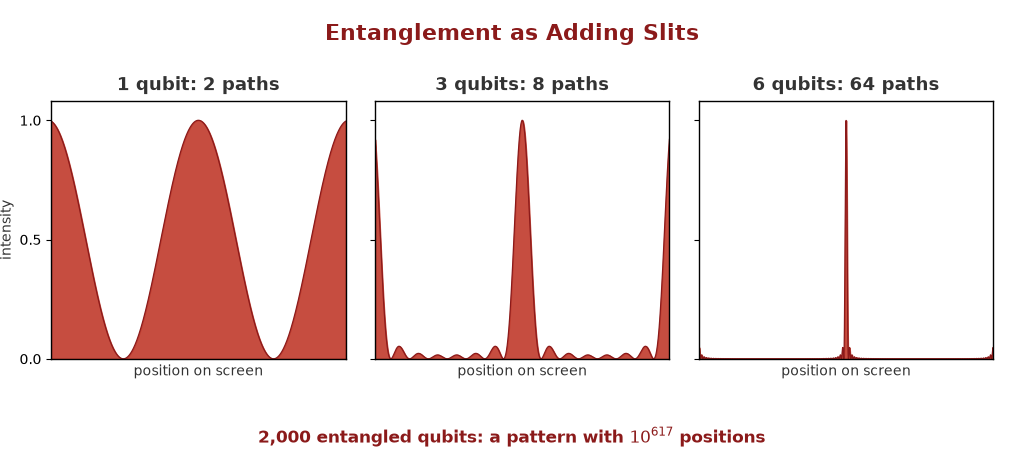
Figure 3. Entanglement as adding slits.

Figure 3. Entanglement as adding slits. Each added qubit doubles the number of paths, and the interference pattern sharpens with every doubling. With enough qubits the pattern has room to encode the answer to a problem with 10^617 candidates.

The Massive Wave: The quantum computer acts as a single, massive wave passing through all of these slits simultaneously. This is why entanglement is the engine of quantum computing. It expands the "solution space" (the back wall) from a simple pattern of black-and-white stripes into a canvas complex enough to reveal the prime factors we are looking for. The Challenge - Fragility: However, maintaining such a system in a delicate state of superposition is extremely hard. The more qubits that are added, the more complex and fragile the system becomes. If any other physical object - air molecules, heat, stray magnetic fields, interacts with the system in this delicate state, the synchronization breaks, the wave collapses, and the complex interference pattern dissolves into noise. This challenge of maintaining the system is known as Coherence. Note on "Logical" Qubits: Throughout this paper, when we discuss the number of qubits required (e.g., 4,000 for encryption), we are referring to Logical Qubits. In the real world, physical qubits are prone to error. To create one perfect "Logical Qubit" that can hold a value without breaking, engineers often need to tie together thousands of "Physical Qubits" to correct for noise. Building a machine with enough physical qubits to create these logical units is the primary engineering challenge of the next decade. Coherence, Decoherence, and Error Correction

VI. Coherence: The Challenge

For superposition, entanglement, and probability shaping to work, the qubits must remain in a delicate state where their quantum properties are not forced to choose a definite value. This fragile condition is known as Coherence. [3] The Environment is a Detector: The problem is that the universe is hostile to these states. Recall from the Double Slit experiment that if a detector "peeks" at the particle, the wave collapses. In a real quantum computer, you don't need a deliberate detector to ruin the experiment. Heat (vibrating atoms) Electromagnetic radiation (WiFi signals) Stray particles (Cosmic rays) All of these act like unintended measurements. Even a single interaction with a stray heat photon effectively asks the qubit, "Are you a 0 or a 1?" When that happens, the qubit is forced to decide. Superposition collapses, entanglement breaks, and the coordinated quantum wave falls apart. The result on our "back wall" is no longer a sharp, high-resolution solution; it reverts to random noise.

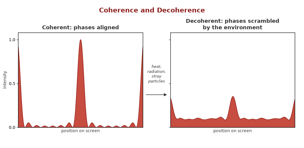
Figure 4. Coherence and decoherence.

Figure 4. Coherence and decoherence. Left: with phases aligned, the interference pattern is sharp enough to read. Right: the same system after the environment has scrambled the phases. The information is not destroyed so much as smeared beyond recovery.

This loss of quantum behavior is called Decoherence. It is not a theoretical limitation, but a physical one. It is the primary engineering challenge standing between today's experimental devices and the quantum machines of the future.

VII. The Solution: Shaping Probabilities

At this point, thanks to entanglement, our quantum computer is holding a vast landscape of possibilities, a "back wall" covered in 10^617 potential answers. But right now, the wave is spread equally. Every answer looks the same. If we measured the system now, we would just get random noise. How do we guide the system toward the one right answer? The Algorithm as a Lens: A quantum computer does not search sequentially. Instead, it uses interference, a controlled method of reshaping the likelihood of different outcomes. To visualize this, we return to the Double Slit Experiment. Imagine placing a series of optical lenses between the slits (the qubits) and the back wall. We haven't looked at the answer yet; we are simply applying these lenses to "bend" the waves passing through the system, adjusting their phases so they focus on a single bright point on the wall. Note: What is the "Lens" made of? In the actual hardware, there are no glass lenses. Instead, engineers use Quantum Gates. These are precise pulses of energy (microwaves or lasers) applied to the qubits. By hitting a qubit with a specific pulse, we rotate its state, mathematically shifting its wave phase. A quantum algorithm is simply a sequence of these pulses designed to create the interference pattern we want. How Do We Shape the Lenses? And how do we know where to place the lenses if we don't know the answer? We use the rules of the problem itself. The lens is built from whatever structure the problem has, and that structure can come from two different places.

Structure from mathematics (the RSA case): Modular exponentiation is periodic. Multiply a number by itself again and again modulo N and the sequence of remainders eventually repeats. The length of that repeat, the period, is hidden, and knowing it is enough to factor N Appendix A. Shor's algorithm builds its lens from this fact. It prepares a superposition over all inputs, applies the periodic function, and then applies a Quantum Fourier Transform, the same operation that decomposes a sound into its component frequencies. Every candidate period that is wrong interferes destructively; the true period reinforces. A reader who knows the Fourier transform from signal processing already knows the engine of Shor's algorithm. [6]

Structure from physics (the molecule case): Consider the challenge of designing a new drug molecule. We may not know the final, stable shape of the molecule, but we do know the physics that govern it. We know that two atoms cannot occupy the same space, and we know that like charges repel, etc. We build these physical constraints into the algorithm. These rules act as the lenses. Destructive Interference (High Energy): Consider a configuration where the molecule is folded so that atoms are crashing into each other. This is physically "impossible" or high-energy. The algorithm uses this physical constraint to shift the wave phases so that these answers cancel out. Constructive Interference (Low Energy): Now consider the configuration where the atoms fit together perfectly, the stable, low-energy shape. The algorithm aligns the waves for this outcome.

Figure 5. Two lenses.

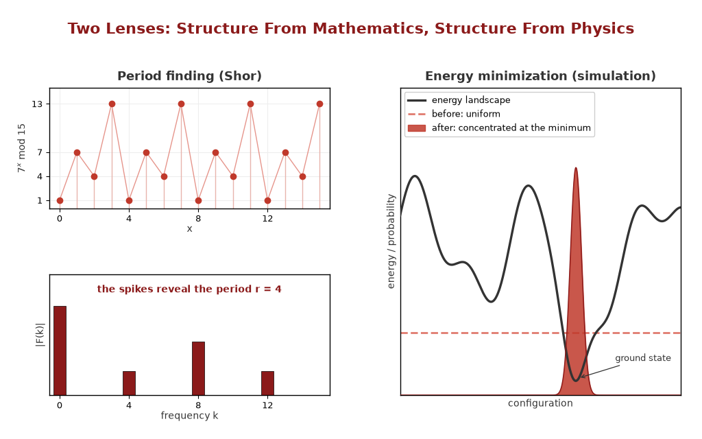
Figure 5. Two lenses. Left: for factoring, the structure is a hidden period in a number sequence, and a Fourier transform reads it out as spikes. Right: for a molecule, the structure is an energy landscape, and interference concentrates probability at its minimum. Different sources of structure, the same mechanism.

The Result: Nature Finds a Way - Nothing is removed explicitly. No configuration is deleted. Instead, the system mimics nature's own tendency to settle into a stable state. When we finally measure the system, we don't find a random result. Because the "stable" wave (the low-energy solution) has been amplified by our lenses, it dominates the probability distribution.

VIII. Limits and Opportunities: What Quantum Computing Can, and Cannot, Do

Quantum computing is powerful, but it is not a magic oracle. It does not work by checking every possible answer simultaneously. For a quantum algorithm to work, the problem must have a hidden mathematical structure, or "Codable Laws", that we can exploit to create interference. You cannot build a lens for a problem that has no shape. Structured Problems: In the RSA encryption example, the system is defined by exact mathematical relationships (prime factors). In the drug discovery example, the system is defined by the forces of physics. We can code these rules into the algorithm to focus the wave on the correct solution. Unstructured Problems: If a problem is truly random (like finding a specific name in an unsorted pile of paperwork), there is no mathematical structure to "focus" on. The wave cannot be focused in a single stroke, and the best a quantum computer can offer is the modest quadratic speedup of Grover's algorithm Appendix D, useful but far from exponential. Because of this, quantum computing is not a universal replacement for classical machines, but a specialized tool for specific domains: Nature's Home Court: Chemistry and Medicine: The most transformative opportunity lies in drug discovery and materials science. At the molecular level, chemistry is quantum mechanical. A classical computer struggles to simulate a drug molecule because it has to approximate the complex quantum behavior using rigid math. A quantum computer doesn't have to approximate. It simulates the molecule by becoming the molecule. [4] It uses its own physics to mirror the physics of the drug. This could accelerate the design of targeted therapies, enabling patient-specific treatments tailored to an individual's molecular profile. Quantum Simulation "Nature isn't classical, dammit, and if you want to make a simulation of nature, you'd better make it quantum mechanical, and by golly it's a wonderful problem, because it doesn't look so easy." - Richard Feynman [7] Imposing Structure: Logistics and Optimization: Problems like global routing or portfolio construction are not physical, but they have mathematical structure (constraints, costs, dependencies) that can sometimes be mapped onto quantum states. Whether that mapping produces a real advantage is unproven. The methods proposed so far offer, at best, the quadratic gains of the Grover family, and a 2021 analysis by Babbush and colleagues argues that quadratic speedups are unlikely to beat classical hardware once the overhead of error correction is counted. [11] This is the domain where claims should be read most carefully.

How Native Is the Problem to the Machine? The three cases above sit on a single gradient, and the gradient is the most useful thing to take from this primer. At one end, the problem and the machine share the same physics. The precise term is isomorphism: the equations governing the molecule and the equations governing the qubits have the same form, so one can stand in for the other without approximation. The older word is analog. An analog computer is one that is analogous to the problem, as a wind tunnel is to flight or a tide-predicting machine is to the sea, and a quantum simulator is an analog computer built at the level of the physics itself. [12] This is where the exponential claims rest on the firmest ground. Analog Computation and Isomorphism In the middle, the problem is not physical but has hidden mathematical structure, a period or a symmetry, that interference can read directly. Factoring is the clean example. The machine is not being the problem; it is applying a mathematics the problem happens to be written in. At the far end, the problem has no structure the machine can exploit, and the quantum computer is reduced to a faster search engine. The gain is quadratic, and after error correction it may round to nothing.

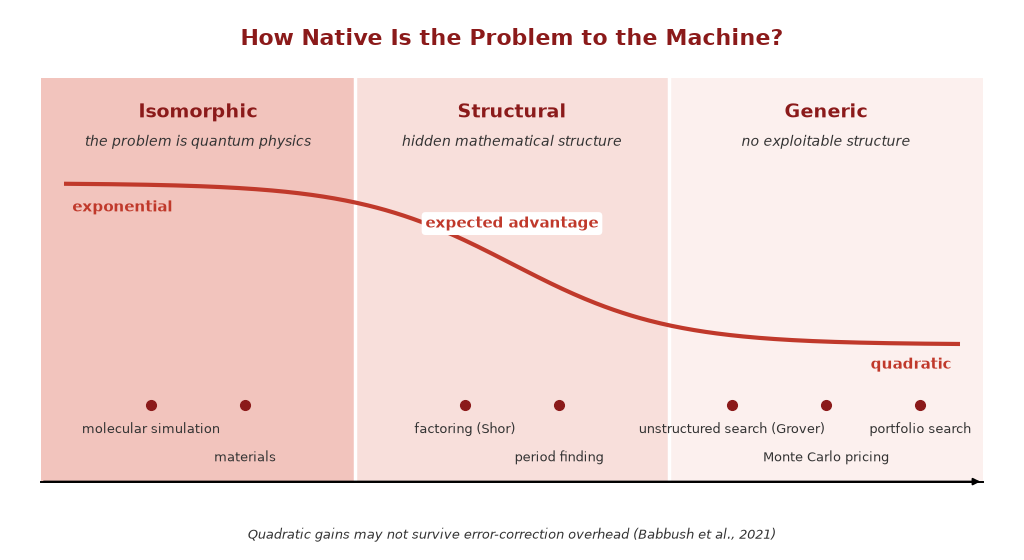
Figure 6. How native is the problem to the machine?

Figure 6. How native is the problem to the machine? Expected advantage falls as the problem moves from isomorphic (the problem is quantum physics) through structural (a hidden mathematical regularity) to generic (nothing to exploit). Most finance applications proposed so far sit at the right.

The practical reading is that the advantage a quantum computer offers is proportional to how native the problem is to it. That is a sharper claim than "quantum computers are faster," and it is the one a reader should carry into any conversation about applications. The Structure Gradient

IX. Conclusion: The Hybrid Architecture

Ultimately, the goal of quantum computing is not to replace classical computers, but to complete them. The emerging model is a Hybrid Architecture where the quantum computer functions as a Specialized Accelerator, similar to a modern GPU (Graphics Processing Unit). [5] Just as a standard CPU offloads heavy graphics or AI tasks to a GPU, future supercomputers will offload specific problems of scale to a QPU (Quantum Processing Unit). Appendix C: The Hardware Race In this workflow, the classical computer retains control over logic, operating systems, and data storage. It only triggers the QPU when it hits a barrier of scale, such as factoring a massive number or simulating a complex molecule. The QPU applies the "lenses" of interference to isolate the solution and returns the result to the classical system. Appendix D: The Software

Figure 7. The hybrid architecture.

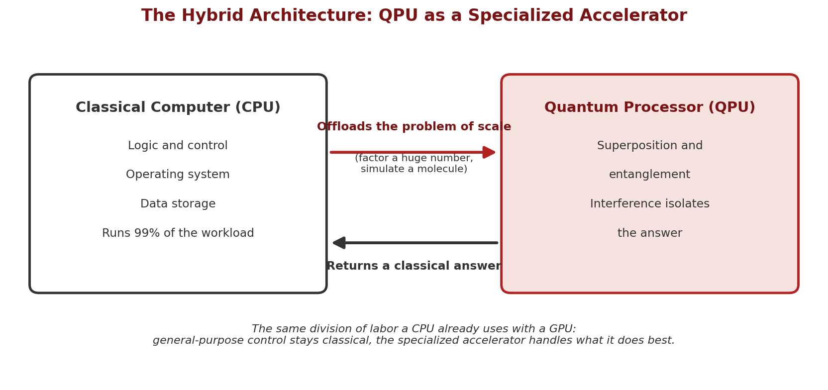
Figure 7. The hybrid architecture. The classical processor keeps control, logic, and storage; the quantum processor is called for the specific subproblem it is native to, and returns a classical answer.

This approach leverages the best of both physical regimes: the rock-solid reliability of classical bits for general computing, and the probabilistic power of qubits for the problems that are simply too big to count. The Hybrid Architecture: QPU as Accelerator

A closing observation connects this primer to a companion essay in this library, From Smooth to Jagged. That essay follows how mathematics grew a new tool each time reality proved rougher than the existing ones could describe. Quantum simulation is where that story reaches a different kind of ending for physical systems. When the model and the system obey the same physics, the mathematics stops being an approximation of the system and becomes a description in the system's own language. The modeling step does not vanish (the Hamiltonian still has to be written down and compiled into gates), but the gap between model and reality closes to engineering overhead. That ending is available only to problems that are themselves physics. For everything else, including the markets that occupy my working days, the gradient in Section VIII still applies, and the mathematics has to keep growing.

References

[1] Rivest, R. L., Shamir, A., & Adleman, L. (1978). "A Method for Obtaining Digital Signatures and Public-Key Cryptosystems." Communications of the ACM, 21(2), 120-126.
[2] Feynman, R. P., Leighton, R. B., & Sands, M. (1965). "Quantum Behavior." In The Feynman Lectures on Physics, Vol. III. Addison-Wesley.
[3] Zurek, W. H. (2003). "Decoherence, einselection, and the quantum origins of the classical." Reviews of Modern Physics, 75, 715.
[4] Cao, Y., et al. (2019). "Quantum Chemistry in the Age of Quantum Computing." Chemical Reviews, 119(19), 10856-10915.
[5] Gambetta, J. (2020). "IBM's Roadmap for Scaling Quantum Technology." IBM Quantum Computing Blog, September 2020.
[6] Shor, P. W. (1994). "Algorithms for quantum computation: discrete logarithms and factoring." Proceedings of the 35th Annual Symposium on Foundations of Computer Science, 124-134.
[7] Feynman, R. P. (1982). "Simulating Physics with Computers." International Journal of Theoretical Physics, 21, 467-488.
[8] Bell, J. S. (1964). "On the Einstein Podolsky Rosen paradox." Physics Physique Fizika, 1(3), 195-200.
[9] Dirac, P. A. M. (1930). The Principles of Quantum Mechanics. Oxford University Press.
[10] Grover, L. K. (1996). "A fast quantum mechanical algorithm for database search." Proceedings of the 28th Annual ACM Symposium on Theory of Computing, 212-219.
[11] Babbush, R., McClean, J. R., Newman, M., Gidney, C., Boixo, S., & Neven, H. (2021). "Focus beyond Quadratic Speedups for Error-Corrected Quantum Advantage." PRX Quantum, 2, 010103.
[12] Lloyd, S. (1996). "Universal Quantum Simulators." Science, 273(5278), 1073-1078.

The four appendices of the original paper (RSA mathematics, entanglement and Bell's theorem, the hardware race, and key algorithms) now live as notes in this library, linked from the text above. The full paper with appendices is available for download.