Hurst Exponent and Fractal Dimension
A first pass. Incomplete by design.
Part of the track Derived, Borrowed, Learned
Fractal dimension
Halve your ruler and the measured length of a smooth line doubles; the area of a filled region quadruples. Measure the coast of Britain with an ever-shorter ruler and its length grows by roughly 2^1.25. The coastline is a 1.25-dimensional object: too wrinkled to be a line, too empty to fill a plane. Mandelbrot's 1967 paper made this measurable rather than metaphorical. The surface of the lungs runs the same trick from the other side, folding a tennis court of area into a chest, with a dimension approaching 3.
Hurst exponent
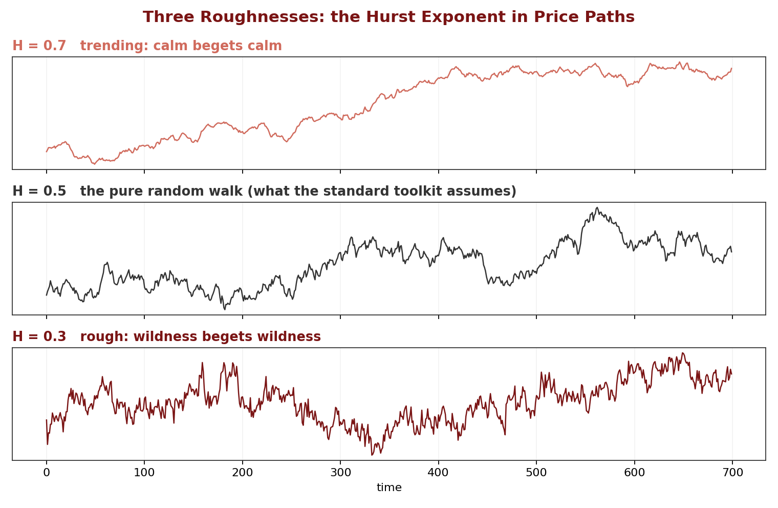
Harold Hurst studied Nile flood records in the 1950s and found that the range of cumulative deviations grew like n^H with H ≈ 0.7 rather than the n^0.5 a random process would give. H measures persistence:
- H = 0.5: increments independent; the random walk.
- H > 0.5: persistent; trends continue.
- H < 0.5: anti-persistent; reversals dominate.
The identity
For a self-affine path (one whose statistics are the same under rescaling), fractal dimension and Hurst exponent are linked by D = 2 − H. The pure random walk's H of 0.5 is its dimension of 1.5. This is why Mandelbrot could move between coastlines and cotton prices with the same tools: both are questions about roughness.
Markets
Bachelier, Black-Scholes, and most of the standard toolkit assume H = 0.5 and thin tails. Mandelbrot's claim was that real price series live at some other roughness: volatility clusters, and the pattern is self-similar across time scales. The claim was eventually measured for volatility itself, with H near 0.1. See Rough VolatilityNoteSeedRough VolatilityGatheral, Jaisson, and Rosenbaum (2018) measured the Hurst exponent of realized volatility across many markets and found values near 0.1. Volatility is far rougher than a Brownian path, and the standard models are the wrong calculus for it.. The consequence for the calculus is in Rough Path TheoryNoteSeedRough Path TheoryLyons (1998): a rough path alone does not determine the integrals along it, so enrich the path with its iterated integrals. Once you do, differential equations driven by paths of any roughness become well defined, with no probability required..
Review log
- 2026-09-08: seeded from Sections V and VI of From Smooth to Jagged.
Appears in
Essays that draw on this note.
- From Smooth to JaggedHow mathematics grew a new tool each time reality posed a problem the existing math could not solve, from Taylor series to the Fourier transform, stochastic calculus, fractal geometry, and rough paths, ending with a personal encounter with Benoit Mandelbrot and its bearing on reading markets.
Links out
- Rough VolatilityGatheral, Jaisson, and Rosenbaum (2018) measured the Hurst exponent of realized volatility across many markets and found values near 0.1. Volatility is far rougher than a Brownian path, and the standard models are the wrong calculus for it.
- Rough Path TheoryLyons (1998): a rough path alone does not determine the integrals along it, so enrich the path with its iterated integrals. Once you do, differential equations driven by paths of any roughness become well defined, with no probability required.
Referenced by
Other notes and pages that link here.
- Brownian Motion and Itô CalculusA path continuous everywhere and differentiable nowhere broke ordinary calculus. Itô's lemma repaired it with one extra term, tuned exactly to Brownian roughness.
- Rough VolatilityGatheral, Jaisson, and Rosenbaum (2018) measured the Hurst exponent of realized volatility across many markets and found values near 0.1. Volatility is far rougher than a Brownian path, and the standard models are the wrong calculus for it.
Related
- Brownian Motion and Itô CalculusA path continuous everywhere and differentiable nowhere broke ordinary calculus. Itô's lemma repaired it with one extra term, tuned exactly to Brownian roughness.
- The Mandelbrot SetIterate z → z² + c and ask whether the orbit stays bounded. The boundary between staying and escaping is infinitely intricate, and it is a picture of where prediction fails.